Research Article - Neuropsychiatry (2016) Volume 6, Issue 6
Probability-based prediction model using multivariate and LVQ-PNN for diagnosing dementia
- †Corresponding Author:
- Jiann-Der Lee
Department of Neurosurgery, Chang Gung Memorial Hospital at LinKou
Taoyuan, Taiwan 333; Department of Electrical Engineering
Ming Chi University of Technology, New Taipei City
Taiwan 24301
Tel: 03-2118800, Ext: 5316
Abstract
Objective:
The aim of this study was to develop a prediction model that integrated various image features and neuropsychological scores to yield a single estimate reflecting the probability of dementia.
Method:
A total of 130 subjects belong to Normal control group, AD group, and MCI group, were recruited in this study. For these subjects, the multiple features obtained from different modalities, including structural MRI morphometry (volume / shape), rs-fMRI, and neuropsychological assessment measures (NPA) were used to explore an optimal set of predictors of conversion from MCI to AD. Unlike previous studies using logistic regression analysis, a new method based on learning vector quantization (LVQ) and probabilistic neural network (PNN) is proposed to establish a prediction model.
Results:
We test the baseline, 1-year follow-up, and 2-year follow-up scans of 17 AD subjects (M/ F=5/12), 22 normal controls (NC; 13/9), 16 subjects that remain stable MCI (MCI-s; 11/5), and 4 subjects convert to AD within a given timeframe (MCI-c; 2/2). This study found that the proposed quantitative indicator provides well-behaving AD state estimates, corresponding well with the actual diagnosis.
Conclusion:
According to the results, all of the test data have the trend that decreased over time. It has the potential to establish an effective decision support and data visualization framework for improving AD diagnostics, allowing clinicians to rapidly analyze large quantities of diverse patient data and as a screening measure and evaluated tool in therapeutic trials.
Keywords
Mild cognitive impairment, Alzheimer’s disease, Multivariate-based prediction model, LVQPNN
Introduction
According to the report [1], thirty millions of people suffer from dementia and, as a consequence of the aging population, the number of people that will be affected is expected to double every 20 years. It is noted that the majority of dementia cases are caused by Alzheimer’s disease (AD). AD is a progressively neuro-degenerative disorder characterized by leading to deficit of cognitive functions, such as memory loss and cognitive degeneration, and behavioral impairment, resulting in declining quality of daily life [2]. Since AD is irreversible and there is no cure, current treatment focuses on lessening its symptoms. Therefore, how to diagnose AD accurately in early stage has become increasingly significant. Additionally, prediction of the conversion from Mild Cognitive Impairment (MCI) to AD is one of major topics in AD research. Mild cognitive impairment (MCI) is a transitional stage between normal aging and demented status. The syndrome is defined by the greater cognitive decline than other age and educational matched individuals, but no interference of daily function. According to the major symptoms, MCI is characterized with memory loss and cognitive impairment.
It is known that MCI has been associated with a risk for AD because of similar structural brain changes [3-5]. Therefore, detection of brain changes that reflect pathological processes of MCI would prevent or postpone degeneracy either from normal to MCI or from MCI to AD. If MCI can be diagnosed at early stage and effective intervened, then it is possible to reduce the advanced damages. To achieve this goal, various neuroimaging methods have been proposed to examine the predictive abilities with respect to AD and other dementia illnesses [6-10]. For example, single photon emission computed tomography (SPECT) and positron emission tomography (PET) are often used with the aim of achieving early diagnosis. However, under the consideration of imaging cost and non-invasive requirement, magnetic resonance imaging (MRI) has been widely used for early detection and diagnosis of MCI and AD [11-13].
Brain atrophy typically starts in the medial temporal and limbic areas, subsequently extending to parietal association areas and finally to frontal and primary cortices. Early changes in hippocampus, amygdala, and entorhinal cortex have been demonstrated with the help of MRI and these changes are consistent with the underlying pathology of MCI and AD. Methods based on volumetric measurements [14-16], or on visual rating scales [17] have largely been used to assess cortex atrophy. Hippocampal volumes and entorhinal cortex measures have been found to be equally accurate in distinguishing between AD and normal cognitive elderly subjects [18]. However, the segmentation and identification of hippocampus or entorhinal cortex are usually time-consuming and prone to interrater and intra-rater variability. In addition, the enlargement of ventricles is also a significant characteristic of AD due to neuronal loss. Ventricles are filled with cerebro-spinal fluid (CSF) and surrounded by gray matter (GM) and white matter (WM). As a result, by measuring the ventricular enlargement, hemispheric atrophy rate shows higher correlation with the disease progression.
In addition to the atrophy of brain regions, neuropsychological assessment (NPA) has featured prominently over the past 30 years in the characterization of dementia associated with Alzheimer disease (AD) [19,20]. As research has increasingly focused on earlier stages of illness, it has become clear that biological markers of AD can precede cognitive and behavioral symptoms by years, such as Mini Mental State Examination (MMSE) [21] and Clinical Dementia Rating scale (CDR) [22], the Cognitive Abilities Screening Instrument (CASI) [23], trail making test A (TMT-A) and B (TMT-B) [24], etc.
Functional MRI (fMRI) is a neuroimaging technique that is presumed to directly link specific cognitive activity to neurophysiological changes, such as functional cerebral hemodynamics. In fMRI-based studies on the blood oxygen level dependent (BOLD) contrast, have shown that cognitively intact older individuals that demonstrate a greater degree of activation in many literatures [25-29]. Therefore, it appears that fMRI activation might be predictive of future cognitive decline during the prodromal stages of AD and MCI. The resting state functional MRI (rs-fMRI) of the brain is measured by spontaneous low frequency fluctuations in BOLD signal patterns across anatomical regions. A correlation of these low frequency fluctuating time courses, generated by their spontaneous activity, can be used to establish the degree of functional connectivity (FC) between regions. Examination of rs-fMRI connectivity might be an even more useful technique for observing the initial functionally related changes that occur in AD and prior to behavioral manifestations [30,31].
In clinical diagnosis, physicians often rely on subjective sense and experience to judge the type of disease and conditions, and therefore, prone to have different diagnostic results between different physicians. The derived diagnostic system can then be used either to assist the physician when diagnosing new patients in order to improve the diagnostic speed, accuracy and/or reliability, or to train students, physicians, non-specialists to diagnose patients in a special diagnostic problem. The most important mission of any diagnostic system is the process of attempting to determine and/or identify a possible disease or disorder and the decision reached by this process. For this purpose, machine learning algorithms are widely employed [32,33]. For these machine learning techniques to be useful in medical diagnostic problems, they must be characterized by high accuracy, the ability to deal with ambiguous cases, the transparency of diagnostic knowledge, and the ability to explain decisions. Previous studies have utilized different techniques such as principal components analysis (PCA), linear discriminant analysis (LDA), support vector machines (SVM), and orthogonal partial least squares (OPLS) for multivariate data analysis [34-39].
Generally speaking, there is no single test to determine if someone has dementia. Clinicians diagnose Alzheimer’s and other types of dementia based on a careful reading of the medical history, a physical examination, laboratory tests, and the characteristic changes in medical images, day-today function and behavior associated with each type. Doctors can determine whether a person has dementia with a high level of certainty. But it is hard to determine the exact type of dementia because the symptoms and brain changes of different dementias can overlap. Therefore, in this study, we develop a prediction model to estimate the probability of dementia based on multivariate and learning vector quantization (LVQ) combined with probabilistic neural network (PNN). A single estimate reflecting the probability of dementia can provide a classification and positions the patient into a continuous space between the values -1 and 1, indicating a patient’s disease state in relation to previously known control (healthy) and positive (disease) populations. This makes it possible to assess the disease severity, i.e. it is not simply a yes or no diagnosis.
Methods
▪ Participants
According to the research [40], most patients with AD were aged at 65 or older. Therefore, most of the subjects in the whole data we choose were ranged over 65 years old. The image data used in this study were provided by Chang Gung Memorial Hospital, Lin-Kou, Taiwan. The degree of clinical severity for each participant was evaluated by experienced clinicians conducted independent semi-structured interviews which included a set of questions regarding the functional status of the participant, along with a standardized neurologic, psychiatric, and health examination. This interview generates an overall Clinical Dementia Rating (CDR) and Mini Mental State Examination (MMSE) score. Demographic information is provided in Table 1.
| Group | Normal control | MCI | AD |
|---|---|---|---|
| Individuals (Male/Female) Mean age (yrs) Education time (yrs) MMSE scores |
40 (23/17) 63.85 ± 5.86 10.20 ± 4.30 28.43 ± 1.17 |
62 (26/36) 68.35 ± 6.36 7.31 ± 4.57 25.49 ± 4.24 |
28 (11/17) 69.43 ± 8.14 6.46 ± 4.98 16.11 ± 5.21 |
Table 1: Demographic data and cognitive scores.
▪ Neuropsychological assessment features
Neuropsychological assessment is an evaluation of cognition, mood, personality, and behavior that is conducted by licensed clinical neuropsychologists. The most beneficial factor of neuropsychological assessment is that it provides an accurate diagnosis of the disorder for the patient when it is unclear to the psychologist what exactly he / she have. This allows for accurate treatment later on in the process because treatment is driven by the exact symptoms of the disorder and how a specific patient may react to different treatments. In the past, the researches [19-20] confirmed that NPA scores could provide more accurate and specific guidelines for the diagnosis of AD dementia and MCI due to AD. In this study, each participant received the following neuropsychological measures.
(1) Memory: Wechsler Memory Scale-III (mainly Logical Memory and Visual Reproduction subtests) Word Sequence Learning Test, and Benton Visual Retention Test.
(2) Language: Object Naming Test and Semantic Association of Verbal Fluency.
(3) Visuospatial function: Three- Dimensional Block Construction and Judgment of Line Orientation.
(4) Executive Function: Modified Card Sorting Test, Trail Making Test part B, and Color Trail Test.
(5) Attention: Trail Making Test part A, and Digit Span and Digit Symbol Substitution subtests of WAIS-III.
Detailed demographics and performance on standard neuropsychological tests of patient groups is listed in Table 2, a summary of the neuropsychological tests from all participants. Domains of cognitive functions are assessed, including memory, executive function, language and visual-spatial skills. Subjects with depression are excluded by using Hamilton Depression Scale for NC group and Cornell Scale for Depression in Dementia in patient groups (AD, and MCI). MCI: mild cognitive impairment; AD: Alzheimer’s disease; MMSE: Mini-mental State Examination; WCST: Wisconsin Card Sorting Test; SD: standard deviation.
| NPA score | NC | MCI | AD |
|---|---|---|---|
| Mean Global score (SD) | |||
| MMSE (maximum, 30) | 28.23 ± 1.30 | 25.10 ± 3.87 | 15.07 ± 6.34 |
| Word sequence learning-recall | 3.17 ± 1.93 | 0.45 ± 0.74 | 0.04 ± 0.20 |
| Visual reproduction II | 11.60 ± 3.09 | 8.57 ± 2.80 | 6.23 ± 1.86 |
| Logic Memory II | 11.60 ± 2.72 | 7.97 ± 3.72 | 3.15 ± 1.87 |
| Semantic Assocation of Verbal Fluency | 33.40 ± 6.82 | 29.57 ± 6.03 | 14.55 ± 6.20 |
| WCST-S Completed Categories | 5.20 ± 1.13 | 3.69 ± 1.77 | 1.88 ± 2.76 |
| WAIS-III Digit Symbol-scaled | 10.37 ± 2.55 | 9.52 ± 2.95 | 6.94 ± 2.71 |
| WAIS-III Digit Span-scaled | 11.30 ± 2.76 | 10.54 ± 2.65 | 7.67 ± 2.16 |
| 3-D Block Construction Models | 28.6 ± 0.77 | 27.27 ± 3.1 | 18.41 ± 10.50 |
| Object Naming Test | 16.00 ± 0.00 | 15.97 ± 0.18 | 13.13 ± 3.65 |
Table 2: Statistical data of neuropsychological assessment scores.
▪ Feature selection
To obtain the required features, a lot of image processing algorithms including segmentation and interpolation are used to obtain volume and shape features from magnetic resonance images (MRI). The whole-brain MRI scans are obtained by a 3-Tesla MR scanner (Magnetom Trio with TIM system, Siemens, Erlangen, Germany). T1- weighted images are acquired by magnetizationprepared 180 degrees radio-frequency pulses and rapid gradient-echo (T1-MPRAGE) series. The following imaging parameters are used: repetition time (TR)=2000ms, echo time (TE)=4.16 ms, and flip angle=9 degrees. The results are represented as a 224×256 matrix, and slice thickness=1mm in 160 slices. T2-weighted fluid-attenuated inversion-recovery (FLAIR) images are acquired to rule out concomitant neurological disorders. Imaging parameters of the T2 FLAIR sequence are used: repetition time (TR)=9000ms, echo time (TE)=85 ms, and inversion time (TI)=2500 ms. Number of slices=34, slice thickness=4 mm. The total acquisition time for both sequences is 6 minutes 34 seconds. BOLD rs-fMRI data are acquired in four runs lasting four minutes each by means T2*-weighted echo planar imaging (EPI) free induction decay (FID) sequences applying the following parameters: TR=1671 ms, TE=35 ms, matrix size=64×64, field of view (FOV)=256 mm, in-plane voxel size=4 × 4 mm, flip angle=75 degrees, slice thickness=4mm and no gap. Functional volumes are consisted of 30 trans-axial slices. All subjects are asked to relax, stay awake, and don’t need to do anything [41].
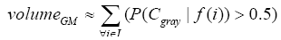
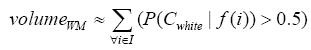
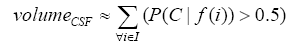
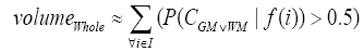
More specifically, to obtain the volume feature, a set of MRI data was registered to a standard spatial coordinate system, i.e., Talairach coordinate system [42]. Therefore, each voxel is thus comparable with the other registered MRI or a reference template. The normalization herein is performed by using a 12-parameter affine transform and a Bayesian framework to a T1-weighted MRI template, provided by ICBM, NIH P-20 project [43]. The volumes of brain tissues such as GM, WM and CSF indicate important information, especially in brain degeneration diseases [44]. A clustering-based segmentation algorithm provided by SPM8 [45] is adopted to extract GM, WM and CSF probability maps from the original MRI data. The value of each voxel in the corresponding probability map indicates the posterior of the voxel belonging to the tissue by giving its gray intensity. As a result, we can calculate the volumes of GM, WM, CSF and the whole brain by the following equations:
 (1)
(1)
 (2)
(2)
 (3)
(3)
 (4)
(4)
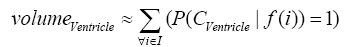
where i is any pixel of the MRI data and f(i) stands for the gray level of i. Next, binary ventricle volume data, M(x, y, z), are extracted from MR images using a region growing algorithm with a threshold, which is estimated through a double threshold algorithm. After thresholding, the binary ventricle regions are obtained by using fill, erosion and dilation operations. The edges of the binary images are detected by Sobel operation on a slice-by-slice manner. The segmented region is then represented as a binary mask image M, where 1 stands for the ventricle pixel and 0 stands for the non-ventricle pixel. Therefore, Eq. (5) is used to measure the cerebral ventricle, as shown in Figure 1 (a) and (b).

Figure 1: (a) CSF binary map, (b) ventricle mask image, and (c) edges of (b).
 (5)
(5)
where i is any pixel of the mask data , M is mask image and f(i) stands for the gray level of i.
Since the volume features extracted from the whole 3-D volume cannot capture the variation of the anatomical shape, Wang [46] proposed a shape-based classification method to obtain 3-D and 2-D shape features. To obtain the feature of 3-D shape, we used a leave-one-out method to construct training set and testing set. Three sets of probability map were then built by using Eq. (6) and as shown in Figure 2.

Figure 2: (a) Probability of normal controls, (b) probability of patients and (c) discriminate map.
 (6)
(6)
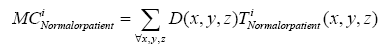
Where t indicates the type of the subjects, comprising normal, AD and MCI, M is the number of training samples, and I stand for the grey level of the ventricular mask image. Next, we obtained a discriminate map by subtracting the normal probability map from the patient probability map, as shown in Figure 2 (c). Lastly, a matching coefficient (MC) between a testing input and the discriminate map can be calculated using Eq. (7). Where D(x,y,z) is the discriminate map and T stands for the testing ventricular mask image.
 (7)
(7)
Through the above image processing algorithms, we obtained individual volume and shape features. The definition of shape features is listed in Table 3. In order to confirm whether there is a significant effect of the classification for these features, we use statistical one-way analysis of variance (ANOVA) to compare differences between three groups on various features (continuous variables). Initially, all of five volume features and eighteen shape features extracted individually from all participants are used in ANOVA test. Finally, three volume features and seventeen shape features as shown in Table 4 are retained. Although the features adopted have statistical significance (< 0.05) between three groups, some of features may be redundant or have highly correlation. Therefore, we employed the linear and nonlinear feature dimensionality reduction methods including of principal component analysis (PCA) [47] and Isomap [48] to achieve this goal. More details of these image processing algorithms can be found in [49,50].
| Shape features | Description |
|---|---|
| Matching coefficient | Similarity measure between each input dataand the discriminant map |
| Area | Area of ventricle |
| Perimeter | Perimeter of ventricle |
| Compactness | Square of the perimeter divided by area |
| Elongation | The ratio of height and width of a rotatedminimal bounding box covered whole ventricle |
| Rectangularity | Area of ventricle divided by area of rotatedminimal bounding box |
| Symmetry | The similarity between right and left ventricle |
| Axis shape descriptors | The distances from ventricle’s centroid to four corner points |
| Minimum thickness | The minimum distance between ventricle’s right side point setand left side point set |
| Mean signature value | 1D expression of ventricle’s edge |
Table 3: List of shape features.
| Features | Mean volume ± S.D. | |||||
|---|---|---|---|---|---|---|
| Volume | Normal | MCI | AD | p-value (NC vs. MCI) |
p-value (NC vs. AD) |
p-value (MCI vs. AD) |
| VGM VWM VCSF |
873.6 ± 47.7 634.9 ± 37.5 849.4 ± 107.1 |
837.5 ± 63.1 599.3 ± 30.0 921.3 ± 131.6 |
792.8 ± 89.2 543.5 ± 79.1 988.2 ± 138.6 |
0.018 0.022 0.026 |
0.005 0.026 0.019 |
0.039 0.031 0.020 |
| Features | Mean value ± S.D. | |||||
| Shape | Normal | MCI | AD | p-value (NC vs. MCI) |
p-value (NC vs. AD) |
p-value (MCI vs. AD) |
| Area | 1883.2 ± 267.4 | 1989.6 ± 374.5 | 2437.5 ± 655.0 | 0.029 | 0.032 | 0.035 |
| Area (PR) | 682.0 ± 119.7 | 876.3 ± 125.7 | 924.6 ± 176.8 | 0.023 | 0.014 | 0.029 |
| Area (PL) | 678.9 ± 125.0 | 878.2 ± 131.8 | 930.5 ± 181.9 | 0.030 | 0.017 | 0.031 |
| Area (FR) | 164.2 ± 121.5 | 245.3 ± 164.1 | 273.8 ± 182.7 | 0.023 | 0.011 | 0.034 |
| Area (FL) | 168.0 ± 93.1 | 262.3 ± 150.3 | 283.3 ± 179.8 | 0.031 | 0.018 | 0.030 |
| Perimeter | 231.4 ± 28.5 | 269.7 ± 24.0 | 291.6 ± 25.4 | 0.028 | 0.014 | 0.028 |
| Circularity | 47.2 ± 5.1 | 39.7 ± 3.1 | 37.5 ± 2.9 | 0.028 | 0.016 | 0.026 |
| Elongation | 1.4 ± 0.7 | 1.3 ± 0.4 | 1.2 ± 0.3 | 0.019 | 0.006 | 0.024 |
| Rectangularity | 0.6 ± 0.1 | 0.7 ± 0.3 | 0.7 ± 0.2 | 0.028 | 0.024 | 0.037 |
| d(A,G) | 35.4 ± 1.8 | 38.0 ± 4.1 | 40.8 ± 4.4 | 0.040 | 0.029 | 0.044 |
| d(B,G) | 37.2 ± 2.5 | 40.6 ± 4.2 | 42.8 ± 5.3 | 0.029 | 0.032 | 0.040 |
| d(C,G) | 39.1 ± 3.8 | 42.3 ± 3.2 | 43.6 ± 4.2 | 0.041 | 0.034 | 0.042 |
| d(D,G) | 35.0 ± 2.3 | 38.1 ± 1.8 | 43.2 ± 3.7 | 0.022 | 0.022 | 0.030 |
| d(A,C) | 74.6 ± 5.0 | 81.2 ± 7.9 | 84.4 ± 8.3 | 0.009 | 0.010 | 0.021 |
| d(B,D) | 72.9 ± 5.1 | 79.4 ± 4.8 | 83.6 ± 8.4 | 0.017 | 0.005 | 0.023 |
| Min thickness | 26.7 ± 2.9 | 29.7 ± 2.3 | 31.4 ± 3.1 | 0.016 | 0.008 | 0.017 |
| Mean Sig. | 26.4 ± 3.0 | 27.4 ± 2.9 | 29.2 ± 3.7 | 0.037 | 0.021 | 0.047 |
Table 4: Statistical analysis of features.
▪ Multivariate-based prediction model
The main aim of this study is to develop a comprehensive, integrated image and neuropsychological assessment scores prediction model, which would yield a single estimate representing the probability of dementia. Unlike other studies [51-53] using logistic regression to estimate the prediction model, we adopt learning vector quantization combined with probabilistic neural network to establish the desired prediction model. The proposed model does not calculate an optimal cutoff point that yields the best ratio between true positive and false negative, instead it will provide a continuous outcome to indicate the probability of dementia. Although a dichotomous outcome produced by different type of classifier would appear to make clinical diagnosing easier, it would loss important information. Moreover, identifying individuals with MCI at high risk of conversion to AD is of great importance to clinicians, the individuals, and their families and for selecting appropriate subjects for therapeutic trials. Therefore, this predictive model would also be useful as a screening measure in therapeutic trials by selecting subjects more likely to decline cognitively and functionally and thus be more likely to benefit from treatment. Here, prediction model was accomplished with LVQ-PNN and its detail is described as below.
Basically, the probabilistic neural network (PNN) represents a parallel implementation of a Bayes strategy for pattern classification. Bayes strategies for pattern classification rely on procedures that minimize the “expected risk” of misclassification. The main problem in using Bayes strategies for classification is the estimation of the probability density functions relative to each class. This task is usually accomplished by using a set of training patterns with known classification. A consistent estimate of a multivariate probability density function can be obtained by using the product of univariate kernels. In the particular case of the Gaussian kernel, the multivariate estimate of the probability density function of category A can be expressed as follows:
 (8)
(8)
where i is the current pattern index, m is the total number of training patterns, XAi is the ith training pattern from category θA, σ is a smoothing parameter, and p is the dimensionality of the input space.
The structure of a typical PNN in the case of a two-category problem is shown in Figure 3, where the input layer consists of simple fanout units, and there is one pattern unit for each training pattern in the second layer. Each pattern unit performs a dot product of the input pattern vector X with a weight vector Wi, i.e., Zi=X·Wi and then performs the nonlinear operation:

Figure 3: The probabilistic neural network (PNN).
 (9)
(9)
Assuming X and Wi are normalized to one unit length, which is equivalent to each exponentiation of Eq. (8). The summation units (one each category) simply sum the outputs from all pattern units of the relative class. In the twocategory case there is one output unit and a twoinput unit, which produces a binary output with only a single variable weight C, defined as Eq. (10)
 (10)
(10)
where nA and nB are the numbers of training patterns from categories θA and θB, respectively. If the numbers of training samples from the different categories are in proportion to their a priori probabilities and class losses li do not reflect any bias in the decision, C may simplify to -1. The network is trained by setting the Wi, weight vector in one of the pattern units, equal to each X pattern in the training set and then connecting the pattern unit output to the appropriate summation unit.
PNN possess a very good, Bayes-like classification performance. Unfortunately, if large training sets are available, the computational cost associated with the testing phase of the PNN is much higher than that of the training phase and will become incompatible with real time classification tasks. In order to overcome this inconvenience, learning vector quantization (LVQ) is employed here because it is computationally extremely light and the convergence is reasonably fast. Figure 4 illustrates the flowchart of LVQ.

Figure 4: The flowchart of LVQ.
In summary, the modified version of the PNN proposed here maintains the basic structure of Figure 3, but the number of nodes assigned to each class in the second layer is no longer equal to the number of training patterns of that class; instead, it equals to the number of processing elements per class of the LVQ, as shown as Figure 5.

Figure 5: The modified LVQ-PNN.
Here, the prediction model is accomplished with LVQ-PNN as described above. For each data point randomly selected from input space, the closest prototype (weight) is determined by Eq. (11):
 (11)
(11)
where μj is a set of prototypes, xt is a set of input vector, and αt is a learning ratio. Maximum likelihood of pattern X is computed by Eq. (12).
 (12)
(12)
where d denotes dimension of pattern X, σ is smoothing parameter, and Na denotes total number of samples in class a. After individual feature variables are used to calculate multivariate probability density function through Eq. (12), we selectively summarize the output calculated from pattern (hidden) unit. Summary unit that accumulate the output corresponding to the same kind of training samples, is determined by Eq. (13).
 (13)
(13)
Finally, through the way of competition with each other and winner takes all to obtain the optimized output, defined as
 (14)
(14)
where wji denotes ith connecting weight from j,th neuron, u represents the input corresponding with wji. Then comparing the weighted sum of each competition unit, the one having the highest sum of the inputs is determined to be the winner. This single estimate represents the probability of dementia we hope to obtain. All estimates are reassigned to range [-1, 1].
Results and Discussion
Unlike previous approaches which employed machine learning techniques using data collected in one time slot to predict various AD stages, the statistical technique of longitudinal data analysis is used to compare certain variables of the same participants at different time slots. The longitudinal data are defined as the data resulting from the observations of subjects (human beings, animals, or laboratory samples, etc.) which are measured repeatedly over time [51-54]. The purpose of conducting a longitudinal study is to look at the change of treatments across a time period. That is, by collecting data over time, it can separate changes over time within an individual sample from the differences between subjects at baseline. Thus, these longitudinal studies can give tremendous information on the subjects. The main advantage of the longitudinal statistical design is the fact that the subject group stays the same, with its main goal to keep as many variables as constant as possible. Therefore, by analyzing and comparing within-group statistics in different time slots, we can find the differences in features over time.
In the experiments, we evaluated whether a quantitative indicator can be used as a screening measure for therapeutic trials or not. We tested the baseline, 1-year follow-up, and 2-year follow-up scans of 17 AD subjects (M/F=5/12), 22 normal controls (NC; 13/9), 16 subjects that remain stable MCI (MCI-s; 11/5), and 4 subjects convert to AD within a given timeframe (MCI-c; 2/2). 12 NCs (M/F=8/4), 8 patients with MCI-s (M/F=6/2), and 9 patients with AD (M/F=3/6) are included in the training cluster. The other data are assigned to the testing cluster. From the results, with volume and shape features, we observed that both MCI and AD patient groups exhibit significant statistical differences at different time-points, especially in the CSF volume, where there is a clear upward trend. Hence, all of seventeen features can be used to describe the change over time in this study. Same analysis methods are also used in NPA features. The performance of normal controls shows no significant differences. The MCI patients also do not exhibit significant differences in long-term research. But all of the NPA scores do reflect statistically significant differences in AD group over time. So, all of ten NPA features can be used to describe the change over time in this study. There are three volume features, seventeen shape features, and ten NPA features used in this study. We also added features of rs-fMRI, including twenty-two rs-fMRI (Z-score) features and ten VBM (F-score) features in the experiments. The rs-fMRI, which is a technique used to image intrinsic functional brain connectivity, is considered a promising biomarker for AD as functional brain changes are thought to precede structural brain changes. Many cross-sectional studies have found the differences of functional connectivity (FC) in the brain’s default mode network (DMN) between aging, MCI, and AD. In this study, we looked at the possible changes in FC occurring longitudinally over time, with the aim of assessing the potential usefulness of this technique as a biomarker for disease progression in these three groups.
The baseline and longitudinal changes of the PCC (posterior cingulate cortex) connectivity are assessed to clarify the neural mechanism of these three groups. In patients with AD, connectivity at baseline is decreased in the posterior default mode areas and increased in frontal regions in comparison with NCs. However, at follow-ups, patients show decreased connectivity throughout the entire DMN. These results suggest that within the DMN, hyperconnectivity precedes hypo-connectivity of a certain brain region, and this may signal the early phase of brain dysfunction. It is also noted that the observed connectivity changes follow the trajectory of neuropathology which affects the medial temporal lobe first, followed by the posterolateral cortical regions and, in the latest stages, the frontal cortex. We observe that FC between the hippocampus and a set of regions that were disrupted in MCI, including of frontal lobe, bilateral temporal lobe and insular. Besides, the posterior cingulate cortex, precuneus, hippocampus, caudate and right occipital gyrus show increased connectivity to the hippocampus in MCI. Several regions showed decreased connectivity to the hippocampus over time. These longitudinal results may indicate reduced integrity of hippocampal cortical memory network in MCI.
We explore the whole brain’s condition of atrophy and to examine if it is altered in dementia by the course of time. In MCI patients progressing toward AD, atrophy has been observed, including of temporal, parietal, and frontal lobe. These regions are involved in a number of processes related to cognitive functions and memory retrieval. If they start to atrophy, in simple terms, imply they are suffering from dementia. These results suggest that when we make long-term following study, we can use these results as for important factors to predict the progress of disease and survival over time. In order to evaluate whether these multimodality features change over time can be used as a screening measure, a predictive model that adopts these features as input for analysis is necessary and helpful.
Figure 6 shows the predicted probability of the validation data set. The visualization clearly discloses how predictors contribute to the AD state, facilitating a rapid interpretation of the information. We can find that the quantitative indicator provides well-behaving AD state estimates, corresponding well with the actual diagnoses. All test data have the trend decreased over time. We also can observe the score will be lower than 0.483 after suffering from dementia except for MCI patients. Comparing to the result obtained in a previous classification-based paper [49], it is observed that most of MCI patients has obvious discrimination with NCs. It is implied that these time-oriented features are useful to evaluate which of these cases belong to which group. Especially when comparing with other classification-based methods, this model does not require a physician’s gold standard, so it can allow clinicians to rapidly analyze large quantities of diverse patient data and assist in preliminary screening.

Figure 6: Predicted probability score of validation data set.
Conclusion
In this study, we developed a comprehensive prediction model by integrating image and neuropsychological assessment scores to yield a single estimate representing the probability of dementia. For a clinically meaningful interpretation, this estimate should not be interpreted on its own, but should be instead weighed against the previous probability of AD, which the clinician derives from interpretation by a combination of history taking, physical examination, neuropsychological evaluation, and neuroimaging. Theoretically, all these factors could be included in a prediction model. However, it is difficult to specify which items are significant. For example, history taking or neuropsychological testing should not be included because neither has reached any form of standardization. Therefore, learning vector quantization combined with probabilistic neural network is proposed to establish prediction model and provide a continuous outcome.
According to the results, we found that the quantitative indicator provides well-behaving AD state estimates, corresponding well with the actual diagnoses. All test data exhibit the trend that decreased over time. We hope that this indicator can provide clinicians a useful tool to rapidly analyze large quantities of diverse patient data and as a screening measure in therapeutic trials.
Acknowledgement
The work was partly supported by Ministry of Science and Technology, Republic of China, under Grant NSC98-2221-E-182-040-MY3, MOST104-2221-E-182-052-MY2 and Chang Gung Memorial Hospital with Grant No. CMRPD270053, CMRPD2C0041, CMRPD2C0042, CMRPD2C0043.
References
- Ferri CP, Brayne C. Global prevalence of dementia: a Delphi consensus study.Lancet. Neurology366(9503), 2112-2117 (2005).
- Gauthier S, Reisberg B, Zaudig M,et al.Mild cognitive impairment.Lancet367(9518), 1262-1270 (2006).
- Mattila J, Koikkalainen J, VirkkiA, et al.A disease state fingerprint for evaluation of Alzheimer's disease.J. Alzheimers. Dis 27 (1), 163-176 (2011).
- KlöppelS, StonningtonCM, BarnesJ, et al.Accuracy of dementia diagnosis: a direct comparison between radiologists and a computerized method. Brain 131 (Pt11), 2969-2974 (2008).
- Kawamoto K, Houlihan CA, Balas EA, et al.Improving clinical practice using clinical decision support systems: a systematic review of trials to identify features critical to success. BMJ 330, 1-8 (2005).
- Padilla P, Gorriz JM, Ramirez J, et al.Analysis of SPECT brain images for the diagnosis of Alzheimer’s disease based on NMF for feature extraction. Neuroscience. Letters479(3), 192-196 (2010).
- Chaves R, Ramirez J, Gorriz JM, et al.Alzheimers’s Disease Neuroimaging Initiative, Association rule-based feature selection method for Alzheimer’s disease diagnosis. Exp. Sys. App39(14), 11766-11774 (2012).
- Ramirez J, Gorriz JM, Segovia F, et al.Computer aided diagnosis system for the Alzheimer’s disease based on partialleast squares and random forest SPECT image classification. Neuroscience. Letters472(2), 99-103 (2010).
- Gallix A, Gorriz JM, Ramirez J, et al.On the empirical mode decomposition applied to the analysis of brain SPECT images. Exp. Sys. App39(18), 13451-13461 (2012).
- Salas-Gonzalez D, Gorriz JM, Ramirez J, et al.Two approaches to selecting set of voxels for the diagnosis of Alzheimer’s disease using brain SPECT images.Dig. Sig. Proc(21), 746-755 (2012).
- Iglesias JE, Jiang J, Liu CY, et al.Alzheimers’s Disease Neuroimaging Initiative, Classification of Alzheimer’s disease using a self-smoothing operator. Proc. 14th Int. Conf. Med. Image. Computing.Comput. Assist.Intervent(2012).
- Zhang Z, Wang Y, Zhou L, et al.Multimodel classification of Alzheimer’s disease and mild cognitive impairment. Neuroimage55(3), 856-867 (2011).
- Vemuri P, Wiste HJ, Weigand SD, et al.MRI and CSF biomarkers in normal, MCI, and AD subjects: predicting future clinical change. Neurology73(4), 294-301(2009).
- Juottonen K, Laakso MP, Partanen K, et al.Comparative MR analysis of the entorhinal cortex and hippocampus in diagnosing Alzheimer disease. Am. J.Neuroradiol20(1), 139-144 (1999).
- Colliot O, Chetelat G, Chupin M, et al.Discrimination between Alzheimer Disease, Mild Cognitive Impairment, and Normal Aging by Using Automated Segmentation of the Hippocampus. Radiology 248(1), 194-201 (2008).
- Morra JH, Tu Z, Apostolova LG, et al.Automated mapping of hippocampal atrophy in 1-year repeat MRI data from 490 subjects with Alzheimer's disease, mild cognitive impairment, and elderly controls. Neuroimage45(1), s3-s15 (2008).
- Scheltens P, Leys D, Barkhof F, et al.Atrophy of medial temporal lobes on MRI in ‘probable’ Alzheimer’s disease and normal ageing: Diagnostic value and neuropsychological correlates. J. Neurol. Neurosurg. Psychiatry55 (10), 967-972 (1992).
- Kantarci K. Magnetic resonance markers for early diagnosis and progression of Alzheimer's disease. Expert Rev. Neurotherapeutics5(1), 663-670 (2005).
- Salmon DP, Bondi MW. Neuropsychological Assessment of Dementia. Ann. Rev. Psychology60(1), 257-282 (2009).
- Weissberger GH, Salmon DP, Bondi MW, et al.Which Neuropsychological Tests Predict Progression to Alzheimer’s disease in Hispanics. Neuropsychology27(3), 343-355 (2013).
- Folstein M, Folstein SE, McHugh PR. Mini-mental state: a practical method for grading the cognitive state of patients for the clinician. J. Psychiatric. Res 12(3), 189-198 (1975).
- Hughes CP, Berg L, Danziger WL, et al.A new clinical scale for the staging of dementia. Br. J. Psychiatry140(1), 566-572 (1982).
- Ten EL, Hasegawa K, Homma A, et al.The cognitive abilities screening instrument (CASI): a practical test for cross-cultural epidemiological studies of dementia. Int. Psychoger6(1), 45-58 (1994).
- Tombaugh TN. Trail making test A and B: normative data stratified by age and education. Arch. Clin. Neuropsychology19(2), 203-214 (2004).
- Bookheimer SY, Strojwas MH, Cohen MS, et al.Trail making test A and B: normative data stratified by age and education. New England J. Med 343(1), 450-456 (2000).
- Dickerson BC, Salat DH, Bates JF, et al.Medial temporal lobe function and structure in mild cognitive impairment. Ann. Neurol56(1), 27-35 (2004).
- Li SJ, Li Z, Wu G, et al.Alzheimer Disease: evaluation of a functional MR imaging index as a marker. Radiology 225(1), 253-259 (2002).
- Minati L, Chan D, Mastropasqua C, et al.Widespread alterations in functional brain network architecture in amnestic mild cognitive impairment. J. Alzh. Dis 40(1), 213-220 (2014).
- Teipel SJ, Grothe M, Lista S, et al.Relevance of magnetic resonance imaging for early detection and diagnosis of Alzheimer disease. The Med. Clin. North America97(3), 399-424 (2013).
- Fleishera AS, Sherzaid A, Taylor C, et al.Resting-state BOLD networks versus task-associated functional MRI for distinguishing Alzheimer's disease risk groups. NeuroImage47(4), 1678-1690 (2009).
- Rombouts SA, Barkhof F, Goekoop R, et al.Altered resting state networks in mild cognitive impairment and mild Alzheimer's disease: an fMRI study. Human. Brain.Mapp26(4), 231-239 (2005).
- Sajda P. Machine learning for detection and diagnosis of disease. Radiology 8(1), 537-565 (2006).
- Wang S, Summers RM. Machine learning and radiology. Med. Image. Anal 16(5), 933-951 (2012).
- Fan Y, Batmanghelich N, Clark CM, et al.Spatial patterns of brain atrophy in MCI patients, identified via high-dimensional pattern classification. Neuroimage 39(1), 1731-1743 (2008).
- López MM, Ramírez J, Górriz JM, et al.SVM-based CAD system for early detection of the Alzheimer's disease using kernel PCA and LDA. Neurosci. Lett464(1), 233-238 (2009).
- Plant C, Teipel SJ, Oswald A, et al.Automated detection of brain atrophy patterns based on MRI for the prediction of Alzheimer's disease.Neuroimage 50(1), 162-174 (2009).
- Vemuri P, Gunter JL, Senjem ML, et al.Alzheimer's disease diagnosis in individual subjects using structural MR images: validation studies.Neuroimage39(3), 1186-1197 (2008).
- Westman E, Simmons A, Zhang Y, et al.Multivariate analysis of MRI data for Alzheimer's disease, mild cognitive impairment and healthy controls.Neuroimage 54(2), 1178-1187 (2011).
- Cuingnet R, Gerardin E, Tessieras J, et al.Automatic classification of patients with Alzheimer's disease from structural MRI: a comparison of ten methods using the ADNI database.Neuroimage 56(2), 766-781(2011).
- Alzheimer’s disease facts and figures. (2014).
- Biswal B, Yetkin FZ, Haughton VM, et al.Functional connectivity in the motor cortex of resting human brain using echo-planar MRI. Magn. Res. Med34 (4), 537-541 (1995).
- Talairach J, Tournoux P. Co-Planar Stereotaxic Atlas of a Human Brain: Dimensional Proprotional System: An Approach to Cerebral Imaging. Georg ThiemeVerlag (1988).
- Mazziotta JC, Toga A, Evans A, et al.A probabilistic atlas and reference system for the human brain: International Consortium for Brain Mapping (ICBM). Philos. Trans. R. Soc. Lond. B. Biol. Sci356(1412), 1293-322 (2001).
- Fritzsche KH, Wangenheim A, Abdala DD, et al.A computational method for the estimation of atrophic changes in Alzheimer’s disease and mild cognitive impairment.Comput. Med. Imaging. Graph32(4), 294-303 (2008).
- UCL Institute of Neurology.
- Wang J, de Haan G, Unay D, et al.Voxel-based discriminant map classification on brain ventricles for Alzheimer’s disease.Med. Imag7259(1),67-69 (2009)
- Mulder ER, Jong RA, Knol DL, et al.Hippocampal volume change measurement: quantitative assessment of the reproducibility of expert manual outlining and the automated methods FreeSurfer and FIRST. NeuroImage92(1), 169-181 (2014).
- Biswas S, Bowyer KW, Flynn PJ. Multidimensional scaling for matching low-resolution face images. IEEE. Trans.Patt. Anal. Mach. Intellig34(10), 2019-2030 (2012).
- Yang ST, Lee J, Chang T, et al.Discrimination between Alzheimer's disease and Mild Cognitive Impairment Using SOM and PSO-SVM. Comput.Mathem. Methods.Medicine117-126 (2013).
- Yang ST. Diagnosis and prediction of Alzheimer's disease and Mild Cognitive Impairment with long-term multimodality features, Doctoral Dissertation, Chang Gung University, Taiwan (2015).
- Spies PE, Claassen JA, Peer PG, et al.A prediction model to calculate probability of Alzheimer's disease using cerebrospinal fluid biomarkers. Alzheimer’s & Dementia9(3), 262-268 (2013).
- Palmqvist S, Hertze J, Minthon L, et al.Comparison of brief cognitive tests and CSF biomarkers in predicting Alzheimer’s disease in Mild cognitive impairment: six-year follow-up study. PLoS. ONE7 (6), e38639 (2012).
- Vos SJ, Visser PJ, Verhey F, et al.Variability of CSF Alzheimer’s disease biomarkers: implications for clinical practice. PLoS. ONE9(6), e100784 (2014).
- Bijleveld C, Kamp L, Mooijaart A, et al.Longitudinal Data Analysis: Designs, Models & Methods. Sage Publications (1999).